3.1 Lab Exercise: RC Circuit Time Response
In this lab, we will be measuring the time-response of the voltage across a capacitor in an RC circuit. We will apply an input voltage and measure the \(v_o\) response with an NI myRIO single-board computer, export it to a data file, import that data file into Python, plot the data, derive an analytic model, and compare the analytic model to the data.

The objectives of this lab exercise are for students:
- To explore transient circuit response,
- To deepen their understanding of RC circuits,
- To learn to acquire and log data with a single-board computer (myRIO),
- To learn to export the acquired data to Python,
- To model real circuits and compare the theory and experiment, and
- To learn to better plot and export plots in Python.
Materials
The following materials are required for each lab station:
- a PC with LabVIEW installed,
- a myRIO configured with LabVIEW,
- a multimeter,
- a breadboard,
- jumper wires,
- a \(100\) k\(\Omega\) resistor,
- a \(10\ \mu\)F capacitor,
Build the circuit
Use the following procedure to build the circuit.
- Measure and record the actual resistance \(R\) of the resistor and capacitance \(C\) of the capacitor with a multimeter.
Build the RC circuit (sans source) on a breadboard. The capacitor is polarized; that is, it has a positive and a negative terminal. We must take care to connect such capacitors such that the voltage always drops from the positive terminal to the negative terminal. Sometimes this is indicated by a shorter lead and/or a "\(-\)" symbol on the negative side. (In our case "\(-\)" should connect to the ground node.)
Connect the myRIO to power and to your workstation computer via USB. It will be both the voltage source \(V_s\) and measurement of \(v_o\).
We will be using the MSP connector named
Con the side of the myRIO shown in the figure below.

CWith jumper wires, connect the analog output ground channel
AGND(3) to the ground of your circuit (ensure this is connected to the "\(-\)" capacitor terminal).Connect the analog output channel
AO0(4) to the resistor such that the analog voltage supplied viaAO0andAGNDis applied across both the resistor and capacitor. You now have \(V_s\) supplied by analog outputAO0.Connect
AI0-(8) to the circuit's ground.Connect
AI0+(7) to the node shared by the resistor and capacitor. You now have a measurement of \(v_o\) on analog inputAI0.
Download and Familiarize Yourself with the Labview Project
The LabVIEW project for this lab is available for download here:
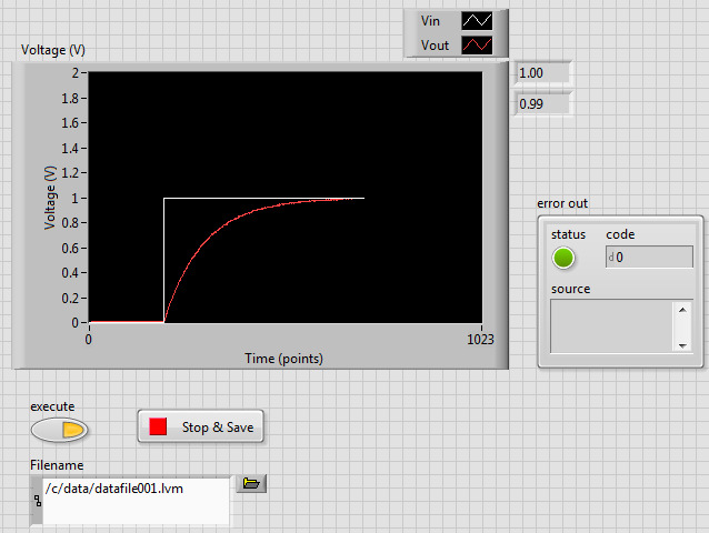
Download the zip file and extract it (you have to actually extract it, not just open it up or a later step won't work). Open the LabVIEW project (not the VI) lab03_RCCircuit.lvproj in LabVIEW. Expand the myRIO device and open the revealed Main.vi program. The front panel of the VI looks as shown in figure 3.
The block diagram of the VI might look as shown in figure 4.
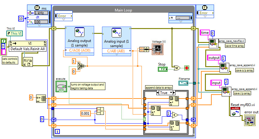
The Main.vi program has the following functionality:
- Outputs an analog voltage of \(1\) V from
AO0when the user toggles a button named execute - Measures the voltage across the capacitor using
AI0+, continuously - Plots the command, output, and input voltages on the same chart, continuously
- Displays digital readouts of the current command, voltage output, and input, continuously
- Uses a timed-loop that executes once every \(10\) ms
- After (and only after) the execute button is pressed, it stores time values (with zero beginning when the button is pressed), measured circuit input voltage \(\widetilde{V}_s\), and measured circuit output voltage \(\tilde{v}_o\) in arrays
- After the timed loop is exited via a Stop & Save button, it writes the three arrays to a LabVIEW
.lvmdatafile on the myRIO via thearray_save_newfile.viandarray_save_append.vifunctions
The code that precedes the Main Loop resets the controls on the front panel to their default values. The block labeled This VI is the VI Server Reference VI and is found in the Functions > Application Control palette. The block labeled Defaults Vals.Reinit All is the Invoke Node VI and is found in the Functions > Application Control palette. After wiring the VI Server Reference to the input of Invoke Node, right-click on the word Method on the Invoke Node VI and select Method for VI Class>Default Values > Reinitialize All to Default. Finally, the block labeled C is the Close Reference VI and is found in the Functions > Application Control palette.
The Case Structure labeled append data to arrays has a False panel that simply passes through arrays instead of appending to them.
Capture the capacitor voltage response
The following procedure can be used to capture the charging of the capacitor.
- Name your data file on the front panel something like
/c/data/datafile001.lvm. - Run your
Main.vi. You should see a zero voltage \(V_s\) and \(v_0\) reading on the chart. - Click the execute button to begin application of \(V_s\) and data acquisition of \(v_o\).
- Observe the voltage response on the chart. You should observe an exponentially decaying approach of \(\tilde{v}_o\) to \(1\) V.
- Once the voltage has leveled off (at least about \(6 \tau = 6 RC\)), again click the execute button to set the applied voltage to zero.
- Once the voltage has leveled off, click the Stop & Save button on the front panel of the VI.
- Locate the data file saved to the myRIO flash memory.
- Use a web browser to navigate to http://172.22.11.2/files, where the myRIO serves its file system
- Navigate to
/c/data. - Identify and open your data file. Each run, a data file is created (or over-written) here with a name specified on your front panel. Old data files may be present.
- Save your data file to a convenient directory on the computer.
Report Requirements
Write a report on your laboratory activities using the template given.
Include the following plots (use Python to make the plots) for both the charging portion of your data and the discharging portion:
The measured \(\widetilde{V}_s\) and \(\tilde{v}_o\) as functions of time and
The measured \(\tilde{v}_o\) as a function of time overlayed with your theoretical prediction for \(v_o\).
Include all measurements made by hand (e.g. resistance).
Include an analysis of a voltage RC circuit that can be used to produce the theoretical predictions in the plots.
- Include, as always, an abstract, introduction, materials and methods, results, and discussion.
It may be helpful to take pictures during the laboratory procedure. These can be included in your report.
Loading Data into Python
Loading the LVM data file into Python is straightforward. You will need to install the lvm_read package using pip:
pip install git+https://github.com/ricopicone/lvm_readFirst, load the lvm_read package:
import lvm_read
import numpy as np
Place your data file, say datafile001.lvm, in the same directory as your Python script. Load the data using the lvm_read.read() function:
data = lvm_read.read('datafile001.lvm')Now you can access the data using the data variable. It’s pretty messy, so we’ll parse it into a more usable format, an matrix of shape (n_samples, n_channels), where n_channels is 3 for us (time, source voltage, capacitor voltage):
n_samples = len(data[0]['data'])
n_channels = 3
data_array = np.zeros((n_samples, n_channels))  # Initialize data array
for i in range(n_channels):
    data_array[:, i] = [p[0] for p in data[i]['data']]
print(f"Data head:\n{data_array[:5]}")
Data head:
[[0. 1. 0.009766]
[0.01 1. 0.019531]
[0.02 1. 0.029297]
[0.03 1. 0.043945]
[0.04 1. 0.053711]]Here’s an example of how to plot the data:
import matplotlib.pyplot as plt

fig, ax = plt.subplots()
ax.plot(data_array[:, 0], data_array[:, 1], label='Source Voltage')
ax.plot(data_array[:, 0], data_array[:, 2], label='Capacitor Voltage')
ax.set_xlabel('Time (s)')
ax.set_ylabel('Voltage (V)')
ax.legend()
ax.grid(True)
plt.draw()
To plot a theoretical function on the same plot, we could define a function such as the following:
def theretical(t):
    return 1 - np.exp(-t / 1)
Now plot both the theoretical capacitor voltage and the measured voltage together:
fig, ax = plt.subplots()
ax.plot(data_array[:, 0], data_array[:, 1], label='$V_S$')
ax.plot(data_array[:, 0], data_array[:, 2], '.', label='$v_C$ Measured', alpha=0.5, markersize=4, marker='o', markerfacecolor='orange', markeredgecolor='none')
ax.plot(data_array[:, 0], theretical(data_array[:, 0]), label='$v_C$ Theoretical')
ax.set_xlabel('Time (s)')
ax.set_ylabel('Voltage (V)')
ax.legend()
ax.grid(True)
plt.show()