5.2  Lab Exercise: Diode Bridge Circuit

In this lab, we will design and build a full wave bridge rectifier for AC-to-DC conversion. We will capture the time response data with the NI myRIO device, export it to a data file, import that data file into Python, plot the data, derive an analytic prediction, and compare the analytic prediction to the data.

The objectives of this lab exercise are for students:

1. To understand AC-to-DC conversion
2. To deepen their understanding of diode circuits
3. To better learn to acquire and log data with a single-board computer (myRIO)
4. To learn to export the acquired data to Python
5. To model real circuits and compare the theory and experiment
6. To learn to better plot and export plots in Python

Materials

The following materials are required for each lab station:

• A PC with LabVIEW installed
• A myRIO configured with LabVIEW
• An oscilloscope
• A multimeter
• A breadboard
• Jumper wires
• Four 1N914 diodes
• A 1 kΩ resistor
• A 100 μF capacitor

Build the circuit

The full wave bridge rectifier circuit we are building can be represented by the circuit diagram of figure 1.

Use the following steps to build the circuit:

1. Use a function generator as the voltage source. Choose a capacitor of nominal capacitance \(C = 100\) μF and a resistor of nominal resistance \(R_L = 1\) kΩ. Select four 1N914 diodes.

2. Measure and record the actual resistance \(R\) and capacitance \(C\) with a multimeter.

3. Measure each diode voltage drop using the multimeter. The stripe on the diode corresponds to the cathode (the direction toward which current typically flows). The voltage drops should be around 0.6 V.

4. Build the circuit on a breadboard. It should look something like figure 2.

Be cautious with the capacitors---they're polarized! Be sure to connect the - terminal to ground.

Get the Main VI

The LabVIEW VI needed for this lab exercise can be downloaded here:

Download LabVIEW VI

Figure 3 shows how the front panel of your VI might look when the capacitor is disconnected.

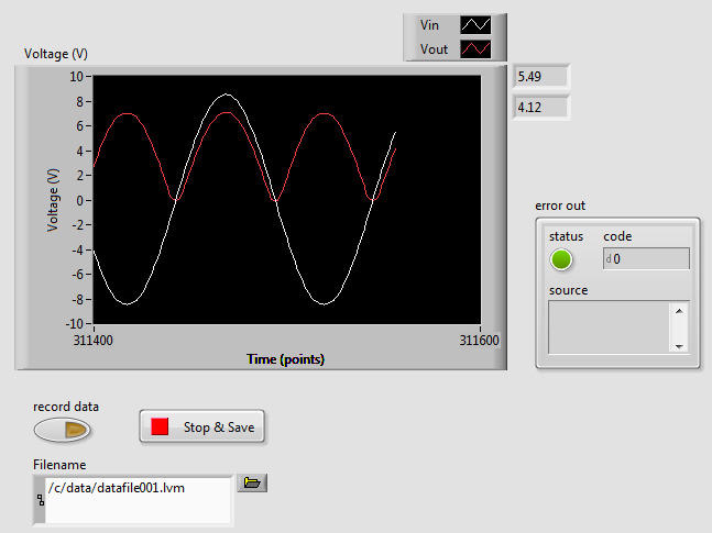
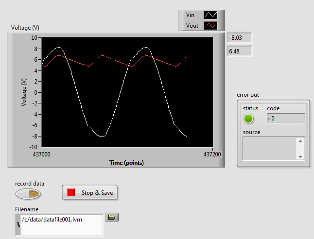
Figure 4 shows how the front panel of your VI might look when the capacitor is connected.

The VI performs the following tasks:

1. Measures the function generator voltage using AI0+, continuously;
2. Measures the voltage across the capacitor using AI1+, continuously;
3. Plots the circuit input (scope output) and circuit output (capacitor) voltages on the same chart, continuously;
4. Uses a timed-loop that executes once every 10 ms;
5. After (and only after) the user toggles the front-panel button record data pressed, stores
   • Time values (with zero beginning when the button is pressed),
   • Measured circuit input voltage \(\widetilde{V}_s\), and
   • Measured circuit output voltage \(\tilde{v}_o\) in arrays; and
6. After the timed loop is exited via a Stop & Save button, write the three arrays to a LabVIEW .lvm datafile on the myRIO via the custom VIs I've written for you array_save_newfile.vi and array_save_append.vi (included in the zip file)

Inspect the back panel of the VI to see how the data is captured, stored, and plotted.

Measure the signals

Use your VI to measure the source voltage \(V_S(t)\) and the output voltage \(v_o(t)\) across the load resistor. To capture data and save it to a file, use the following procedure:

1. (Once your circuit is set up) Run the VI.
2. Click the record data button to start recording data.
3. After a couple seconds, again click the record data button to stop recording data.
4. Edit the filename to reflect the capacitor status and frequency.
5. Click the Stop & Save button to save the data.

You will repeat this procedure for each frequency and capacitor status (i.e., included and excluded). Set your function generator to 8 Vpp.¹ For two cases, the capacitor included and excluded from the circuit, measure and record (save to a data file) each voltage (in and out) over at least three periods of input at 10 Hz.

Repeat for the function generator frequency at the following values:²

• 15 Hz,
• 20 Hz, and
• 25 Hz.

Be sure to note which data file is associated with which frequency. Also, be sure to change the filename after clicking the capture data button twice and before clicking the Stop & Save button.

Without the capacitor, the front panel should display something like what is shown in figure 3. With the capacitor, the front panel should display something like what is shown in figure 4.

Copy your data files to a convenient directory on the computer (e.g. Documents/me316/lab05).

Report requirements

Write a detailed report of your experimental results, as outlined in the report template. Pay special attention to the following.

1. A thorough description of the theoretical analysis of the circuit. As part of this analysis, predict ripple and average DC value for each circuit with the capacitor attached. Also predict the current supplied to the load resistor \(R_L\). Use these and the model of the quick-and-dirty section to give a predicted DC voltage \(v_{DC}\) and ripple \(\Delta v_o\).

2. Four figures that compare each of the capacitor-attached captured data sets (input and output) to its corresponding analytic prediction. It is acceptable to predict only the ripple range and average value of the output, but a full time-analysis is even more fun! In Python, be sure to use plt.xlim() to scale the x-axis such that around 3--5 periods are visible on each plot (or trim the data). Include somewhere on the plot the approximate measured ripple and DC value. (You can use matplotlib's cursor tools to help with the estimate. "Measure" peak-to-peak and divide by two. Alternatively, use numpy's trapz function to numerically integrate the voltage and divide it by the time duration, which should be an integer multiple of the signal's period, to find its average.)

3. Four figures that display the capacitor-detached input and output data sets. Alternatively (preferably), plot these on the corresponding capacitor-attached data set plots. Carefully label and caption these.

4. The other parameters measured in the lab (e.g. \(R_L\), \(C\)).

5. Be sure to comment on how well your predictions matched the theory.

---

1. If you're using a BK Precision function generator, use your VI to hand-tune the function generator voltage to 8 V.↩︎

2. If you're using a BK Precision function generator, use your VI or the oscilloscope to measure the actual frequency, which you should record.↩︎