3.3 1D PLPM Thermal Analysis of the Experiment
Introducing the Experiment
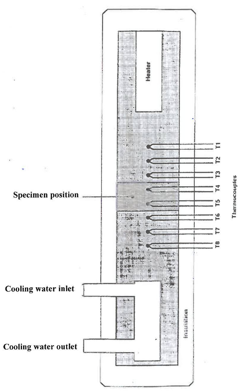
The experimental apparatus by P. A. Hilton (Hilton, 2006; Hilton, 2011) is designed to study linear heat transfer. In figure 1, a cross section of the H112A unit (Hilton, 2011) is shown. At the top we see a heater that supplies heat to the top of an insulated cylindrical rod. At the bottom we see water cooling. Between is a test specimen and 8 thermocouples evenly spaced 15 mm apart, 3 in each of the hot and cold sections, and 2 in the test section. The hot and cold sections of the rod are made of brass. The test section can be exchanged, but for this analysis it will be made of the same brass material at the same diameter of 25 mm as the hot and cold sections. In this experiment, thermal paste is used at interfaces to ensure good thermal contact.
The heater is an electrical resistance that is supplied with variable AC power from the service unit H112 (Hilton, 2006), controlled by a potentiometer (knob labeled "VOLTAGE CONTROLLER") on the front panel, as shown in figure 2. The readings of the current \(i_{\text{RMS}}\) and voltage \(v_{\text{RMS}}\) on the front panel are in RMS, so the average power dissipated in the resistive heater is \(P = i_{\text{RMS}} v_{\text{RMS}}\). All of the dissipated power (units W) is heat transferred through the rod; that is, \(\dot{q} = P\). The maximum voltage is 240 V, although the automatic power shutdown that prevents overheating will begin to interfere with the experiment at higher power levels.
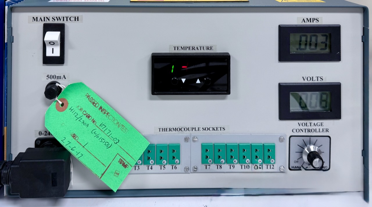
Although we won't use this feature, the H112A thermocouples can be connected to the sockets and corresponding temperature readings can be displayed on the front panel of the service unit.
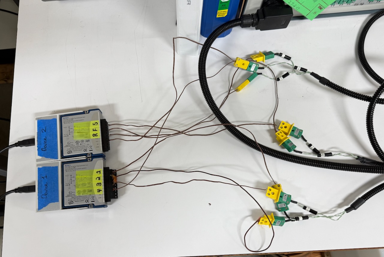
Instead of capturing the thermocouple readings with the service unit, we will use two NI 9211 data loggers, shown in figure 3, connected via USB to a PC running LabVIEW.
Analyzing the Experiment
We will use a 1D partial lumped-parameter model (PLPM) to analyze the experiment. 1D conduction can be modeled analytically using the heat equation, which is a partial differential equation (PDE) that describes the distribution of heat in a given region over time. However, the heat equation is difficult to solve analytically for complex geometries and boundary conditions, and PDE solutions are beyond the scope of most undergraduate courses. Using PLPM, we can derive a set of linear ordinary differential equations (ODEs) that describe the temperature distribution in the rod as a function of time. These can be solved analytically, but we will instead use an easy-to-use numerical ODE solver available in Python's SciPy library.
The Finite Elements
We segment the rod into \(n\) finite elements, each of length \(\delta x\), as shown in figure 4, which has rotated the rod.

We will model each finite element as a lumped capacitance \(C_i\) connected by thermal resistors \(R_i\) and, in most cases, \(R_{i-1}\), to neighboring elements. The leftmost element has the heat transfer rate source \(\dot{q}_S\) entering the system. The rightmost element has the temperature source \(T_S\) (sink, as it were), which will model for us the free-stream temperature of the cooling water. The rightmost conduction resistance \(R_n\) has only half the length of the other resistors. The resistance \(R_{n+1}\) models the convection between the rod and the cooling water.
The Linear Graph Model
We will use a linear graph modeling approach. Consider the linear graph shown in figure 5.

Variable Definitions
We define variables as follows:
- Primary Variables: \(T_{C_1}\), \(T_{C_2}\), ..., \(T_{C_n}\), \(T_{R_{n+1}}\), \(\dot{q}_{R_1}\), \(\dot{q}_{R_2}\), ..., \(\dot{q}_{R_n}\)
- Secondary Variables: \(\dot{q}_{C_1}\), \(\dot{q}_{C_2}\), ..., \(\dot{q}_{C_n}\), \(\dot{q}_{R_{n+1}}\), \(T_{R_1}\), \(T_{R_2}\), ..., \(T_{R_n}\)
- State Variables: \(T_{C_1}\), \(T_{C_2}\), ..., \(T_{C_n}\)
- Vectors: \[\bm{x} = \begin{bmatrix} T_{C_1} \\ T_{C_2} \\ \vdots \\ T_{C_n} \end{bmatrix}, \qquad \bm{u} = \begin{bmatrix} \dot{q}_S \\ T_S \end{bmatrix}, \qquad \bm{y} = \bm{x}.\]
Elemental, Continuity, and Compatibility Equations
Now we are ready to write the equations for the system. The elemental equations are as follows:
\[\begin{align} C_1 &: \dot{T}_{C_1} = \frac{1}{C_1} \dot{q}_{C_1} \\ C_2 &: \dot{T}_{C_2} = \frac{1}{C_2} \dot{q}_{C_2} \\ \vdots &\phantom{:} \vdots \\ C_n &: \dot{T}_{C_n} = \frac{1}{C_n} \dot{q}_{C_n} \\ R_1 &: \dot{q}_{R_1} = \frac{1}{R_1} T_{R_1} \\ R_2 &: \dot{q}_{R_2} = \frac{1}{R_2} T_{R_2} \\ \vdots &\phantom{:} \vdots \\ R_n &: \dot{q}_{R_n} = \frac{1}{R_n} T_{R_n} \\ R_{n+1} &: T_{R_{n+1}} = \dot{q}_{R_{n+1}} R_{n+1} \end{align}\]
A continuity equation is required for each passive branch in the normal tree. They are as follows:
\[\begin{align} C_1 &: \dot{q}_{C_1} = \dot{q}_S - \dot{q}_{R_1} \\ C_2 &: \dot{q}_{C_2} = \dot{q}_{R_1} - \dot{q}_{R_2} \\ \vdots &\phantom{:} \vdots \\ C_n &: \dot{q}_{C_n} = \dot{q}_{R_{n-1}} - \dot{q}_{R_n} \\ R_{n+1} &: \dot{q}_{R_{n+1}} = \dot{q}_{R_n} \end{align}\]
A compatibility equation is required for each passive link (element not in the normal tree). They are as follows:
\[\begin{align} R_1 &: T_{R_1} = T_{C_1} - T_{C_2} \\ R_2 &: T_{R_2} = T_{C_2} - T_{C_3} \\ \vdots &\phantom{:} \vdots \\ R_n &: T_{R_n} = T_{C_n} - T_S - T_{R_{n+1}} \end{align}\]
This is a set of \(4 n + 2\) linear algebraic and differential equations and \(4 n + 2\) unknown variables.
Reducing to the State-Space Model
We can systematically reduce the system of equations to a set of \(n\) first-order differential equations in the state variables of \(\bm{x}\) by eliminating non-state and non-input variables, as follows.
We begin by substituting the continuity and compatibility equations into the elemental equations, eliminating a secondary variable with each substitution. This will eliminate half of the unknown variables and equations. The substitutions yield the following set of equations:
\[\begin{align} C_1 &: \dot{T}_{C_1} = \frac{1}{C_1} (\dot{q}_S - \dot{q}_{R_1}) \\ C_2 &: \dot{T}_{C_2} = \frac{1}{C_2} (\dot{q}_{R_1} - \dot{q}_{R_2}) \\ \vdots &\phantom{:} \vdots \\ C_n &: \dot{T}_{C_n} = \frac{1}{C_n} (\dot{q}_{R_{n-1}} - \dot{q}_{R_n}) \\ R_1 &: \dot{q}_{R_1} = \frac{1}{R_1} (T_{C_1} - T_{C_2}) \\ R_2 &: \dot{q}_{R_2} = \frac{1}{R_2} (T_{C_2} - T_{C_3}) \\ \vdots &\phantom{:} \vdots \\ R_n &: \dot{q}_{R_n} = \frac{1}{R_n} (T_{C_n} - T_S - T_{R_{n+1}}) \\ R_{n+1} &: T_{R_{n+1}} = \dot{q}_{R_n} R_{n+1} \end{align}\]
The equations for \(C_1\) to \(C_n\) can become the state equations by eliminating \(q_{R_i}\) via substitution of the \(R_1\) to \(R_n\) equations. Most of these substitutions are straightforward, but the substitution for \(\dot{q}_{R_n}\) requires two steps. Substituting the \(R_{n+1}\) equation into the equation for \(R_n\) yields can eliminate \(T_{R_{n+1}}\) as follows:
\[ \dot{q}_{R_n} = \frac{1}{R_n} (T_{C_n} - T_S - \dot{q}_{R_n} R_{n+1}). \]
Solving for \(\dot{q}_{R_n}\) yields:
\[ \dot{q}_{R_n} = \frac{1}{R_n + R_{n+1}} (T_{C_n} - T_S). \]
The substitutions are now straightforward and yield the following set of state equations:
\[\begin{align} \dot{T}_{C_1} &= \frac{1}{C_1} \left(\dot{q}_S - \frac{1}{R_1} (T_{C_1} - T_{C_2}) \right) \\ \dot{T}_{C_2} &= \frac{1}{C_2} \left( \frac{1}{R_1} (T_{C_1} - T_{C_2}) - \frac{1}{R_2} (T_{C_2} - T_{C_3}) \right) \\ \vdots &\phantom{:} \vdots \\ \dot{T}_{C_n} &= \frac{1}{C_n} \left( \frac{1}{R_{n-1}} (T_{C_{n-1}} - T_{C_n}) - \frac{1}{R_n + R_{n+1}} (T_{C_n} - T_S) \right) \end{align}\]
Combining terms yields
\[\begin{align} \dot{T}_{C_1} &= \frac{1}{C_1} \left(\dot{q}_S - \frac{1}{R_1} (T_{C_1} - T_{C_2}) \right) \\ \dot{T}_{C_2} &= \frac{1}{C_2} \left( \frac{1}{R_1} T_{C_1} - \left(\frac{1}{R_1} + \frac{1}{R_2}\right) T_{C_2} - \frac{1}{R_2} T_{C_3} \right) \\ \vdots &\phantom{:} \vdots \\ \dot{T}_{C_n} &= \frac{1}{C_n} \left( \frac{1}{R_{n-1}} T_{C_{n-1}} - \left( \frac{1}{R_{n-1}} + \frac{1}{R_n + R_{n+1}} \right) T_{C_n} + \frac{1}{R_n + R_{n+1}} T_S \right) \end{align}\]
The State-Space Model in Standard Form
The state equation has standard form \(\dot{\bm{x}} = A \bm{x} + B \bm{u}\), where \(A\) and \(B\) are matrices containing system parameters. We can transcribe our state equations into this standard form as follows:
\[\begin{align} \begin{bmatrix} \dot{T}_{C_1} \\ \dot{T}_{C_2} \\ \\ \vdots \\ \\ \dot{T_{C_n}} \end{bmatrix} &= \begin{bmatrix} \frac{-1}{R_1 C_1} & \frac{1}{R_1 C_1} & 0 & 0 & \cdots & 0 & 0 & 0 \\ \frac{1}{R_1 C_2} & \frac{-1}{C_2}\left(\frac{1}{R_1} + \frac{1}{R_2}\right) & \frac{1}{R_2 C_2} & 0 & \cdots & 0 & 0 & 0 \\ & & & & & & & \\ \vdots & & \ddots & \ddots & \ddots & & & \vdots \\ & & & & & & & \\ 0 & 0 & 0 & 0 & \cdots & 0 & \frac{1}{R_{n-1} C_n} & \frac{-1}{C_n} \left( \frac{1}{R_{n-1}} + \frac{1}{R_n + R_{n+1}} \right) \end{bmatrix} \begin{bmatrix} T_{C_1} \\ T_{C_2} \\ \\ \vdots \\ \\ T_{C_n} \end{bmatrix} + \\ &+ \begin{bmatrix} \frac{1}{C_1} & 0 \\ 0 & 0 \\ & \\ \vdots & \vdots \\ & \\ 0 & \frac{1}{C_n(R_n + R_{n+1})} \end{bmatrix} \begin{bmatrix} \dot{q}_S \\ T_S \end{bmatrix}. \end{align}\]
The Output Equation in Standard Form
The output equation has standard form \(\bm{y} = C \bm{x} + D \bm{u}\), where \(C\) and \(D\) are matrices containing system parameters. We have said that the output variables are simply \(\bm{y} = \bm{x}\), where \(\bm{x}\) is the state vector, so the output matrix \(C = I_{n \times n}\) is the identity matrix, and the direct transmission matrix \(D = 0_{n \times 2}\) is a zero matrix.
Determining the Parameters
The parameters used in the state-space model are the thermal resistances \(R_i\) and capacitances \(C_i\) of the system. We will try to determine these parameters from the material properties and geometry of the system.
Thermal Capacitance
The lumped thermal capacitance of each element is given by \(C_i = m_i c_i\), where \(m_i\) is the mass of each element and \(c_i\) is the specific heat capacity of the material. For the experiment we will run, the parameters are as follows:
- Mass of each element: \(m_i = \rho_i V_i = \rho_i \pi d_i^2 \delta x/4\), where \(\rho_i\) is the density of the material, \(\rho_i = 8.6 \cdot 10^3 \text{ kg}/\text{m}^3\) (brass).
- Specific heat capacity of the material: \(c_i = 380 \text{ J}/(\text{kg}\cdot\text{K})\) for brass.
Conductive Thermal Resistance
The conductive heat transfer between two adjacent elements in the system has resistance \(R_i\) for \(i = 1, 2, \ldots, n\). Let the length of each element be \(\delta x = L/n\), where \(L\) is the total length of the rod. Then the length between element centers is \(\delta x\). For generality, we allow each element to have a potentially different cross sectional diameter \(d_i\), so that the area \(A_i\) of each element is \(A_i = \pi d_i^2/4\). For each element, we also allow a potentially different thermal conductivity \(k_i\). Therefore the thermal resistance \(R_i\) is given by \[R_i = \frac{\delta x}{k_i A_i} = \frac{4 \delta x}{\pi k_i d_i^2},\] which has units \(\text{K}/\text{W}\). It makes sense that the thermal resistance increases with the length of the element and decreases with the thermal conductivity and cross-sectional area. For the experiment we will run, the parameters are as follows:
- Total length: \(L = 210\) mm
- Diameter (uniform): \(d_i = 25\) mm
- Thermal conductivity (brass): \(k_i = 121 \text{ W}/(\text{m}\cdot\text{K})\)
Convective Thermal Resistance
While most surfaces are insulated, the surface of the rod that is exposed to the flow of water is intentionally subject to convective heat transfer. The average water temperature is given by \(T_S\). The convective thermal resistance \(R_{n+1}\) is given by \[R_{n+1} = \frac{1}{h a},\] where \(h\) is the convective heat transfer coefficient and \(a\) is the surface area of the rod. For the experiment we will run, the parameters are as follows:
- Convective heat transfer coefficient: \(h = 9000 \text{ W}/(\text{m}^2\cdot\text{K})\), based on the flowrate of water and the geometry of the setup
- Surface area of the rod exposed to water: \(a = \pi d^2 / 4\), where \(d = 25\) mm
- Temperature of the water: Record in the lab, but typically around \(20^\circ\text{C}\).
Simulating the Experiment
This script simulates transient heat conduction in a brass rod using finite element analysis. The rod is heated at one end and loses heat to the surrounding environment through convection. We model this as a 1D heat conduction problem with convective boundary conditions. Begin by importing necessary libraries as follows:
import numpy as np
import matplotlib.pyplot as plt
import control
System Parameters
Define the physical properties of the brass rod and the experimental conditions. These parameters are based on typical values for brass and the experimental setup.
L = 0.210  # (m) Length of the rod
di = 0.025  # (m) Diameter of the rod (uniform)
ki = 121  # (W/(m*K)) Thermal conductivity of the rod (brass)
ci = 380  # (J/(kg*K)) Specific heat capacity of the rod (brass)
rhoi = 8.6e3  # (kg/m^3) Density of the rod (brass)
h = 9000  # (W/(m^2*K)) Convective heat transfer coefficient
a = np.pi * di**2 / 4  # (m^2) Cross-sectional area of the rod exposed to convective heat transfer
v = 120  # (V) RMS heater voltage
i = 0.134  # (A) RMS heater current
q = v * i  # (W) Power generated by the heater
Tinf = 20  # (C) Water temperature
Finite Element Discretization
Divide the rod into finite elements and calculate the thermal properties for each element. The finite element method allows us to solve the partial differential equation numerically.
n = 50  # Number of finite elements (increased for better accuracy)
dx = L / n  # Finite element length
Ci = ci * rhoi * np.pi * di**2 * dx / 4  # Thermal capacitance of the finite element
Ri = 4 * dx / (np.pi * ki * di**2)  # Resistance of the finite element
Rn1 = 1 / (h * a)
State-Space Model Construction
Create the state-space matrices A, B, C, and D for the thermal system. This represents the system of ordinary differential equations after spatial discretization.
A = np.zeros((n, n))
for i in range(0, n):
    if i == 0:
        A[0, 0] = -1 / (Ri * Ci)
        A[0, 1] = 1 / (Ri * Ci)
    elif i == n - 1:
        A[n - 1, n - 2] = 1 / (Ri * Ci)
        A[n - 1, n - 1] = -1 / Ci * (1/Ri + 1/(Ri + Rn1))
    else:
        A[i, i - 1] = 1 / (Ri * Ci)
        A[i, i] = -1 / Ci * (1/Ri + 1/Ri)
        A[i, i + 1] = 1 / (Ri * Ci)
Input and Output Matrix Definition
Define how external inputs (heating power and ambient temperature) affect the system and how we observe the system outputs (temperature at each element).
B = np.zeros((n, 2))
B[0, 0] = 1 / (Ci)
B[-1, 1] = 1 / (Ci *(Ri + Rn1))

C = np.eye(n)  # Identity matrix of size n
D = np.zeros((n, 2))
Create Control System Model
Assemble the state-space model using the control systems library. This allows us to easily simulate the system response to various inputs.
sys = control.ss(A, B, C, D)Simulation Function Definition
Create a flexible simulation function that can handle different heating and cooling durations. This allows us to match experimental conditions or explore different heating scenarios.
def simulate(heat_time, cool_time, nt=201):
    """
    Simulate the system response with specified heat and cool times.

    Parameters:
    - heat_time: Duration of heating phase (seconds)
    - cool_time: Duration of cooling phase (seconds)
    - nt: Number of time points for simulation

    Returns:
    - t: Time array (seconds)
    - y_sim: Temperature response array (C), shape (n_elements, n_time)
    """
    total_time = heat_time + cool_time
    t = np.linspace(0, total_time, nt)

    # Create input array
    u = np.zeros((2, nt))
    heat_end_index = int((heat_time / total_time) * nt)
    u[0, :heat_end_index] = q  # Heat input for specified duration
    u[1, :] = Tinf  # Ambient temperature

    # Initial conditions (all elements start at ambient temperature)
    T0 = np.ones(n) * Tinf

    # Run simulation
    y_sim = control.forced_response(sys, t, u, x0=T0).outputs

    return t, y_sim
Temperature Interpolation Function
Create an interpolation function to estimate temperature at any position and time. This is useful for comparing simulation results with experimental sensor data that may not be located at finite element centers.
def simulation_interpolate(time, position, t_sim, y_sim):
    """
    Interpolate the simulation results at given time and position arrays.

    Parameters:
    - time: Time point(s) for interpolation (scalar or array)
    - position: Position(s) along rod for interpolation (scalar or array)
    - t_sim: Time array from simulation
    - y_sim: Temperature response array from simulation

    Returns:
    - Interpolated temperature values
    """
    from scipy.interpolate import interpn

    # Define the grid for interpolation
    # Position grid: center of each finite element
    x_grid = np.linspace(dx/2, L - dx/2, n)

    # Create 2D grid for interpolation (time, position)
    points = (t_sim, x_grid)

    # Transpose y_sim so that rows are time points and columns are positions
    values = y_sim.T

    # Handle scalar vs array inputs
    time_is_scalar = np.isscalar(time)
    position_is_scalar = np.isscalar(position)

    if time_is_scalar and position_is_scalar:
        # Both scalar - single point interpolation
        query_point = np.array([[time, position]])
        result = interpn(points, values, query_point,
                        method='linear', bounds_error=False, fill_value=np.nan)
        return float(result[0])
    elif time_is_scalar:
        # Time scalar, position array
        query_points = np.column_stack([np.full(len(position), time), position])
        result = interpn(points, values, query_points,
                        method='linear', bounds_error=False, fill_value=np.nan)
        return result
    elif position_is_scalar:
        # Position scalar, time array
        query_points = np.column_stack([time, np.full(len(time), position)])
        result = interpn(points, values, query_points,
                        method='linear', bounds_error=False, fill_value=np.nan)
        return result
    else:
        # Both arrays - need to handle broadcasting
        time_mesh, pos_mesh = np.meshgrid(time, position, indexing='ij')
        query_points = np.column_stack([time_mesh.ravel(), pos_mesh.ravel()])
        result = interpn(points, values, query_points,
                        method='linear', bounds_error=False, fill_value=np.nan)
        return result.reshape(time_mesh.shape)
Sensor Position Definition
Define the physical positions of temperature sensors along the rod. These positions match the experimental setup and will be used for predictions.
# Sensor positions (matching experimental setup)
sensor_spacing = 0.015  # (m) Physical spacing between sensors

def get_sensor_positions(n_sensors):
    """Calculate sensor positions for given number of sensors"""
    sensor_start = 45e-3 + L/2 - (n_sensors-1) * sensor_spacing / 2
    return sensor_start + np.arange(n_sensors) * sensor_spacing

# Example with 8 sensors (can be changed as needed)
n_sensors_example = 8
sensor_positions = get_sensor_positions(n_sensors_example)

print(f"Sensor configuration (example with {n_sensors_example} sensors):")
print(f"Sensor spacing: {sensor_spacing*1000:.0f} mm")
print(f"Sensor positions: {sensor_positions*1000} mm")
Sensor configuration (example with 8 sensors):
Sensor spacing: 15 mm
Sensor positions: [ 97.5 112.5 127.5 142.5 157.5 172.5 187.5 202.5] mmExample Simulation
Run a demonstration simulation with typical experimental parameters. This shows the temperature evolution during heating and cooling phases.
# Example simulation parameters
heat_time_example = 2 * 3600  # 2 hours of heating
cool_time_example = 2 * 3600  # 2 hours of cooling

# Run simulation
t_example, y_example = simulate(heat_time_example, cool_time_example)
Temperature Predictions at Sensor Locations
Use interpolation to predict temperatures at the actual sensor positions. This demonstrates how the simulation would compare with experimental measurements.
# Predict temperatures at sensor positions
T_sensor_predicted = np.zeros((len(t_example), n_sensors_example))
for i, t in enumerate(t_example):
    T_sensor_predicted[i, :] = simulation_interpolate(t, sensor_positions, t_example, y_example)
Visualization of Sensor Predictions
Plot the predicted temperature evolution at sensor locations. This shows what we would expect to measure experimentally.
fig, ax = plt.subplots(figsize=(10, 6))

# Define colors for each sensor
colors = plt.cm.tab10(np.linspace(0, 1, n_sensors_example))

# Plot temperature predictions at sensor positions
for i in range(n_sensors_example):
    position_mm = sensor_positions[i] * 1000  # Convert to mm
    ax.plot(t_example / 60, T_sensor_predicted[:, i], color=colors[i],
            label=f'Sensor {i+1} ({position_mm:.0f} mm)', linewidth=2)

ax.axvline(heat_time_example / 60, color='red', linestyle='--', alpha=0.7, label='Heating ends')
ax.set_xlabel('Time (min)')
ax.set_ylabel('Temperature (°C)')
ax.set_title('Predicted Temperature Evolution at Sensor Locations')
ax.grid(True, alpha=0.3)
ax.legend(bbox_to_anchor=(1.05, 1), loc='upper left')
plt.tight_layout()
plt.show()
Temperature Profile Visualization
Show how the temperature profile along the rod changes at different times. This provides insight into the spatial temperature distribution.
fig, ax = plt.subplots(figsize=(10, 6))

# Select specific time points to show profiles
time_points = [0, heat_time_example/4, heat_time_example/2, heat_time_example,
               heat_time_example + cool_time_example/2, heat_time_example + cool_time_example]
time_labels = ['Start', 'Heat 25%', 'Heat 50%', 'Heat End', 'Cool 50%', 'Cool End']

# Define element positions for plotting
element_positions = np.linspace(dx/2, L - dx/2, n)

for i, (t_point, label) in enumerate(zip(time_points, time_labels)):
    t_idx = np.argmin(np.abs(t_example - t_point))
    ax.plot(element_positions * 1000, y_example[:, t_idx], 'o-', label=label)

ax.set_xlabel('Position (mm)')
ax.set_ylabel('Temperature (°C)')
ax.set_title('Temperature Profiles at Different Times')
ax.grid(True, alpha=0.3)
ax.legend()
plt.tight_layout()
plt.show()
Sensor Layout Visualization
Show the relationship between finite elements and sensor positions. This helps understand how interpolation maps simulation results to measurement locations.
fig, ax = plt.subplots(figsize=(12, 6))

# Show finite element positions
element_positions = np.linspace(dx/2, L - dx/2, n)
ax.scatter(element_positions * 1000, np.zeros_like(element_positions),
           marker='|', s=100, c='lightblue', alpha=0.6, label=f'{n} Finite Elements')

# Show sensor positions with different colors
for i, pos in enumerate(sensor_positions):
    ax.scatter(pos * 1000, 0, marker='o', s=20, c=[colors[i]],
               label=f'Sensor {i+1}', alpha=0.9, edgecolors='black', linewidth=1)

ax.set_xlabel('Position (mm)')
ax.set_title('Finite Element Grid and Sensor Positions')
ax.legend(bbox_to_anchor=(1.05, 1), loc='upper left')
ax.grid(True, alpha=0.3)
ax.set_ylim(-0.5, 0.5)
ax.set_ylabel('')
ax.set_yticks([])
plt.tight_layout()
plt.show()
Bibliography
- Hilton, P. A.. "Heat Transfer Service Unit H112: Experimental Operating and Maintenance Manual".
- Hilton, P. A.. "Optional Linear Heat Conduction Unit H112A: Experimental Operating and Maintenance Manual".