4.1  Lab Exercise: Contact Resistance

Purpose

Familiarize students with contact resistance by comparing a thermal joint with no thermal paste to a thermal joint with thermal paste. Students will analyze results to understand how conduction is affected in each situation.

Equipment

• H112 (Hilton, 2006) service unit
• H112A (Hilton, 2011) linear conduction unit
• NI 9211 data loggers (2)
• LabVIEW software
• Heat conducting compound (i.e., thermal paste)
• Solvent for cleaning surfaces (e.g., isopropyl alcohol)

Equipment Details

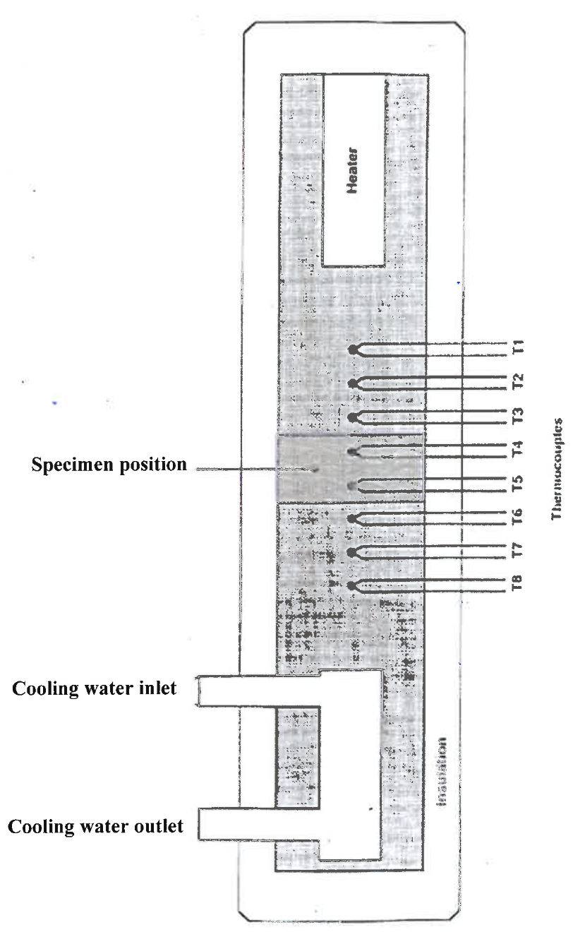
The apparatus is the same as in the linear conduction experiment, shown again in figure 1.

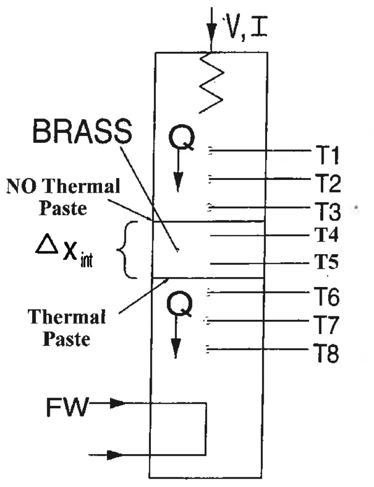
The only difference in the setup is that the upper interface does not have thermal paste applied, as shown in figure 2.

Experimental Procedure

1. Make sure main switch on the H112 is in the off position (no digital display).
2. Turn voltage controller counterclockwise to set AC voltage to minimum. Make sure H112A unit is connected to the service unit H112 via power cord.
3. Connect the closed-loop cooling system to the H112A unit. Turn it on and adjust the temperature controller to room temperature.
4. Release clamps and tension screw on H112A. Ensure the faces of the heated and cooled sections are clean.
5. Only apply thermal paste between the cooled face and intermediate brass section. Do not apply thermal paste between the heated section and intermediate section. Do not clamp the assembly together and leave it unclamped throughout the steps 6 through 10.
6. Turn on main switch. Digital displays will be illuminated.
7. Run the LabVIEW VI to collect temperature data from the data loggers. A sample period of 30 seconds is recommended.
8. Rotate the voltage controller to 120 V.
9. Once the system reaches steady state, rotate turn the voltage controller off and wait for the system to cool to steady-state room temperature.
10. Stop the VI. Check and copy the data file from Documents/LabVIEW Data/ to your own computer.
11. Repeat steps 7 through 10 with the assembly clamped together.
12. When experiment is complete, turn off power by reducing voltage to zero. Allow system to cool before turning off cooling water.
13. Turn off the closed-loop cooling system.
14. Turn off the H112 switch and unplug the electrical supply.
15. Once the system has cooled, wipe off thermal paste from conducting faces.

Lab Report Questions

Review Bergman, Lavine, and Incropera, 2019, section 3.1.4 on contact resistance before proceeding. Within the normal sections of the report, please include the following:

0. Perform a simulation of the experiment. It is very similar to the simulation of the experiment in the previous chapter, but now with two contact resistances inserted into the model between the appropriate elements. Leave the contact resistances as adjustable parameters and tune them to match the experimental data (described below).
1. For each power level, plot the transient temperature measurements versus axial distance for the steady-state temperature distributions.
2. For each power level, plot the steady-state temperature distributions versus axial distance.
3. What do you notice at the thermal joints on the plots?
4. Compute the steady-state temperature slopes for each section:
   1. Hot Section, \(T_1\)–\(T_3\)
   2. Test Section, \(T_4\)–\(T_5\)
   3. Cold Section, \(T_6\)–\(T_8\)
5. Projecting the steady-state temperatures from the slopes, compute the temperature differences across the two interfaces:
   1. \(\Delta T_{HT}\), Hot/Test Interface
   2. \(\Delta T_{TC}\), Test/Cold Interface
6. Compute the total thermal resistance for each of the two interfaces:
   1. \(R_{HT}\) (K/W), Hot/Test Interface
   2. \(R_{TC}\) (K/W), Test/Cold Interface
7. Compute the thermal resistance per unit area for each of the two interfaces:
   1. \(R''_{HT}\) (K/W/m²), Hot/Test Interface
   2. \(R''_{TC}\) (K/W/m²), Test/Cold Interface
8. Using \(R_{HT}\) and \(R_{TC}\) in the simulation model, predict the temperature readings of the sensors through time for each experiment.
9. Plot the predicted temperature readings of the sensors along with the experimental data through time for each experiment.